Data structures
array
An array is a fixed-size collection of elements of the same data type. Elements are stored sequenced in memory.
| Asymptotic computational | |||
|---|---|---|---|
| operation | time | time (bad case) | mem, extra data |
| indexing | O(1) | O(1) | O(n) |
| linear search | O(n) | O(n) | O(1) |
| binary search | O(log(n)) | O(log(n)) | O(1) |
list
An list is a dynamic-size collection of elements of the same data type. Elements are stored sequenced in memory.
It is also known as dynamyc array.
| Asymptotic computational complexity | |||
|---|---|---|---|
| operation | time | time (bad case) | mem, extra data |
| indexing | O(1) | O(1) | O(n) |
| linear search | O(n) | O(n) | O(1) |
| binary search | O(log(n)) | O(log(n)) | O(1) |
| insert | O(n) | O(n) | O(n) |
| delete | O(n) | O(n) | O(n) |
linked list
Linked list is a linear collection of nodes where each node points to the next node.
Unlike an array, the index of an element does not match the physical order in memory.
There are variations of linked lists:
- singly linked list - each node points only to the next element
- doubly linked list - each node points to the next node and to the previous node
- circular linked list - last node points to the first node
- XOR linked list - each node point to the next and previous nodes using the bitwise XOR operation
A circular linked can be used to represent the corners of a polygon, a pool of buffers that are used and released in FIFO ("first in, first out") order, or a set of processes that should be time-shared in round-robin order.
| Asymptotic computational complexity | |||
|---|---|---|---|
| operation | time | time (bad case) | mem, extra data |
| indexing | O(n) | O(n) | O(n) |
| linear search | O(n) | O(n) | O(n) |
| insert | O(1) | O(1) | O(n) |
| delete | O(1) | O(1) | O(n) |
// Example Node structure in Kotlin
class Node<T>{
    var data: T? = null
    var next: Node<T>? = null
    var previous: Node<T>? = null
}
Note. Linked lists are always slower than array-based lists on modern hardware. With array-based lists, elements are stored adjacent to each other in memory. With linked lists, they are not. Adjacent elements in memory can be loaded together into the CPU cache. Elements of linked lists cannot. If data is not in the CPU cache, the CPU has to stop working and wait for the data to be loaded from RAM.
hash table
A hash table is a collection of the key/value pairs. Keys are unique. Several keys may map to the same value.
Pairs are stored in buckets or slots.
Hash function computes index of bucket, where pair with specified key can be found. Ideally, the hash function will assign each key to a unique bucket. But in real world can be collistions, when function generates same index for moew than on key.
In simple case buckets stored as array. But it is not necessary. For example, in Java 8, buckets are stored in linked list. When list too large, list will be transformed to the balanced tree which has O(log n) complexity for add, delete, or get. And when tree too small it will be converted to list. This improves the worst-case performance from O(n) to O(log n).
In many situations, hash tables turn out to be on average more efficient than search trees or any other table lookup structure. For this reason, they are widely used in many kinds of computer software.
Hash table also known as hashmap, dictionary, associative array.
| Asymptotic computational complexity | |||
|---|---|---|---|
| operation | time | time (bad case) | mem, extra data |
| search | O(1) | O(n) | O(n) |
| insert | O(1) | O(n) | O(n) |
| delete | O(1) | O(n) | O(n) |
trees
Tree is a hierarchical collection of nodes in which each node can have zero or more child nodes.
Root is a first node.
Leaf is node without child nodes.
Breadth is the number of leaves.
Sibling nodes are nodes with the same parent.
The height of node is the length of the longest downward path to a leaf from that node. The height of the root is the height of the tree. Conventionally, an empty tree (tree with no nodes) has height −1.
The depth of a node is the length of the path to its root.
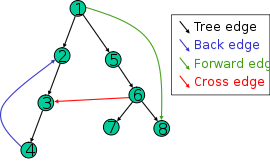
Edge or link is connection between neighboring nodes. There are edges that actually does not belong to the tree:
- back edge points from a node to one of its ancestors
- forward edge points from a node to one of its descendants
- cross edge points from a node to a node that is neither an ancestor nor a descendant
Distance is the number of edges along the shortest path between two nodes.
Level of node is the number of edges along the unique path between it and the root node.
Width is the number of nodes in a level.
There are some kinds of trees:
- binary tree is a tree whose nodes have at most two children.
- balanced tree is a tree where the left and right subtrees' heights of each node differ by at most one.
- red–black tree is a kind of self-balancing binary search tree. Each node stores an extra bit representing "color" ("red" or "black"), used to ensure that the tree remains balanced during insertions and deletions.
- B-tree is self-balancing search tree in which each node can contain more than one key and can have more than two children.
- cartesian tree is a binary tree derived from a sequence of numbers. All numbers are unique. A symmetric (in-order) traversal of the tree results in the original sequence. The parent of any non-root node has a smaller value than the node itself.
- AVL tree is a kind of self-balancing binary search tree.
It uses the balance factor (height(left-subtree) − height(right-subtree)) for each node. When tree unbalanced one of the following rotations can be performed:
- left rotation
- right rotation
- left-right rotation
- right-left rotation
Time complexity of indexing, searching, insertion and deletion operations is O(log(n)). In bad case O(n) for cartesian tree and binary tree, and O(log(n)) for other kinds of trees.
graphs
Graph is a collection of nodes connected by edjes.
Edge is a connection between two nodes.
A directed graph or digraph is a graph in which edges have orientations.
A weighted graph is a graph in which a number (the weight) is assigned to each edge. Weight can represent distance, cost and so on.
A tree is an undirected graph in which any two vertices are connected by exactly one path, or equivalently a connected acyclic undirected graph.
Adjacency matrix is a way to represent graphs.
Let's we have graph with 6 nodes. Then the adjency matrix will be 6x6. First row will indicate neighbors of the first node. Second row will indicate neighbors of the second node, and so on.
For example, an element of the matrix m[0][2] determines whether the node with index 0 is associated with the node with index 2. Similarly, the element m[2][0] determines whether the node with index 2 is associated with the node with index 0.
Typically a value of 0 in an adjacency matrix means that a pair of nodes is not connected. Otherwise, the nodes are associated with a given weight.
As you can see, an adjacency matrix is a symmetric matrix with 0 on main diagonal.
val graph = arrayOf(
            intArrayOf(0, 0, 1, 2, 0, 0, 0),
            intArrayOf(0, 0, 2, 0, 0, 3, 0),
            intArrayOf(1, 2, 0, 1, 3, 0, 0),
            intArrayOf(2, 0, 1, 0, 0, 0, 1),
            intArrayOf(0, 0, 3, 0, 0, 2, 0),
            intArrayOf(0, 3, 0, 0, 2, 0, 1),
            intArrayOf(0, 0, 0, 1, 0, 1, 0)
        )